Violin
R Graph Gallery
Welcome the R graph gallery, a collection of charts made with the R programming language.
Hundreds of charts are displayed in several sections, always with their reproducible code available. The gallery makes a focus on the
tidyverse and ggplot2. Feel free to suggest a chart or report a bug; any
feedback is highly welcome. Stay in touch with the gallery by following it on Twitter
or Github. If you're new to R,
consider following thiscourse.
ggplot2
ggplot2 is the most popular alternative to base R graphics. It is based on the Grammar of Graphics and its main advantage is its flexibility, as you can create and customize the graphics adding more layers to it. This library allows creating ready-to-publish charts easilyCUSTOMIZATION
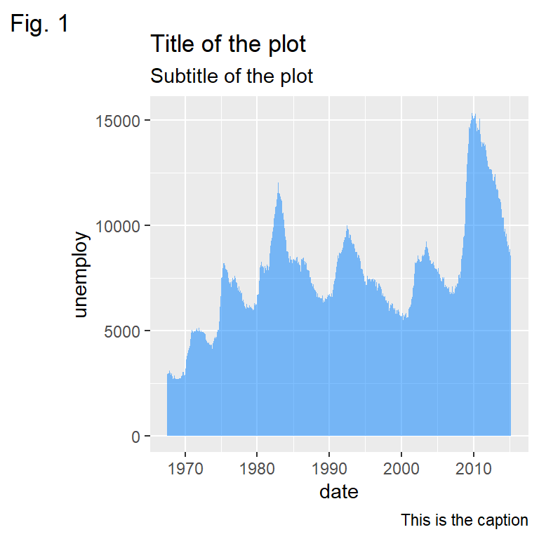
The ggplot2 package allows customizing the charts with themes. It is possible to customize everything of a plot, such as the colors, line types, fonts, alignments, among others, with the components of thethemefunction. In addition, there are several functions you can use to customize the graphs adding titles, subtitles, lines, arrows or texts.Title, subtitle, caption and tag
![Title, subtitle, caption and tag in ggplot2]()
Text annotations
![Text annotations in ggplot2]()
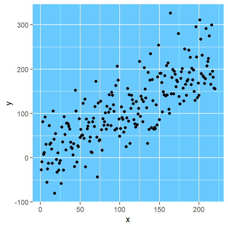
Background color
![Background color in ggplot2]()
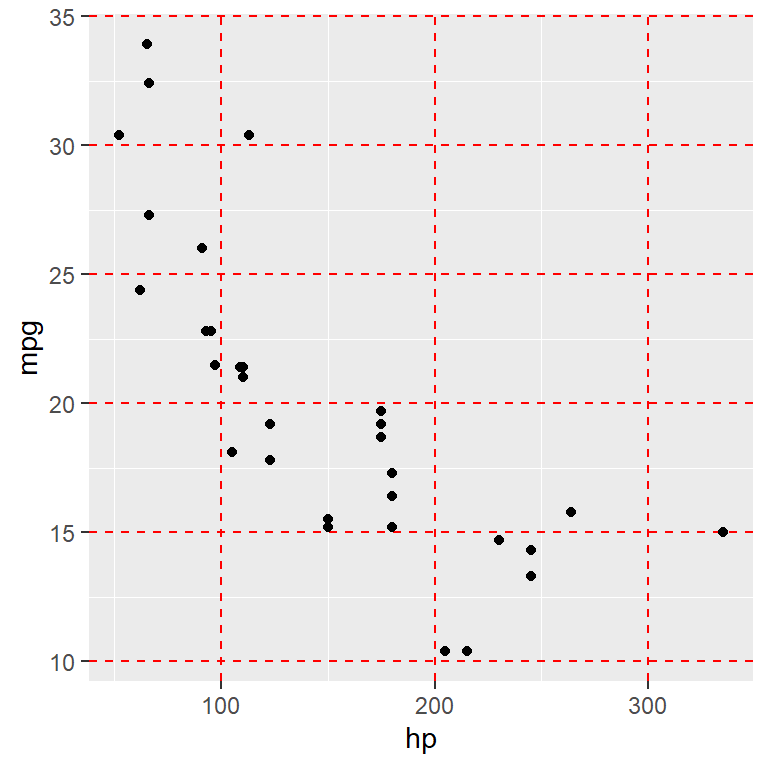
Grid customization
![Grid customization in ggplot2]()
Margins
![Margins in ggplot2]()
Themes
![Themes in ggplot2]()
Legends
![Legends in ggplot2]()
Reference lines, segments, curves and arrows
![Reference lines, segments, curves and arrows in ggplot2]()
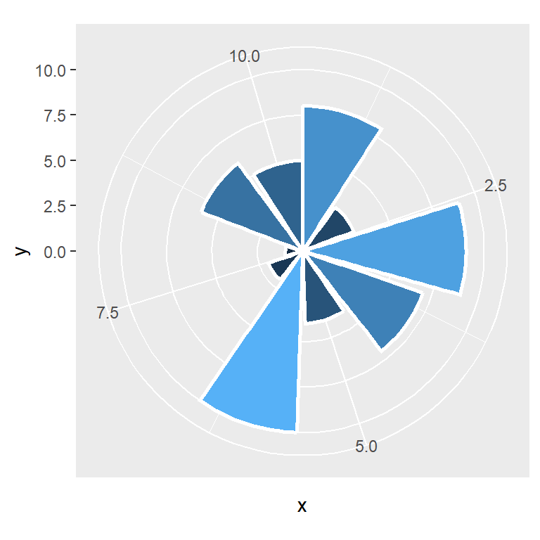
Coordinate systems
![Coordinate systems in ggplot2]()
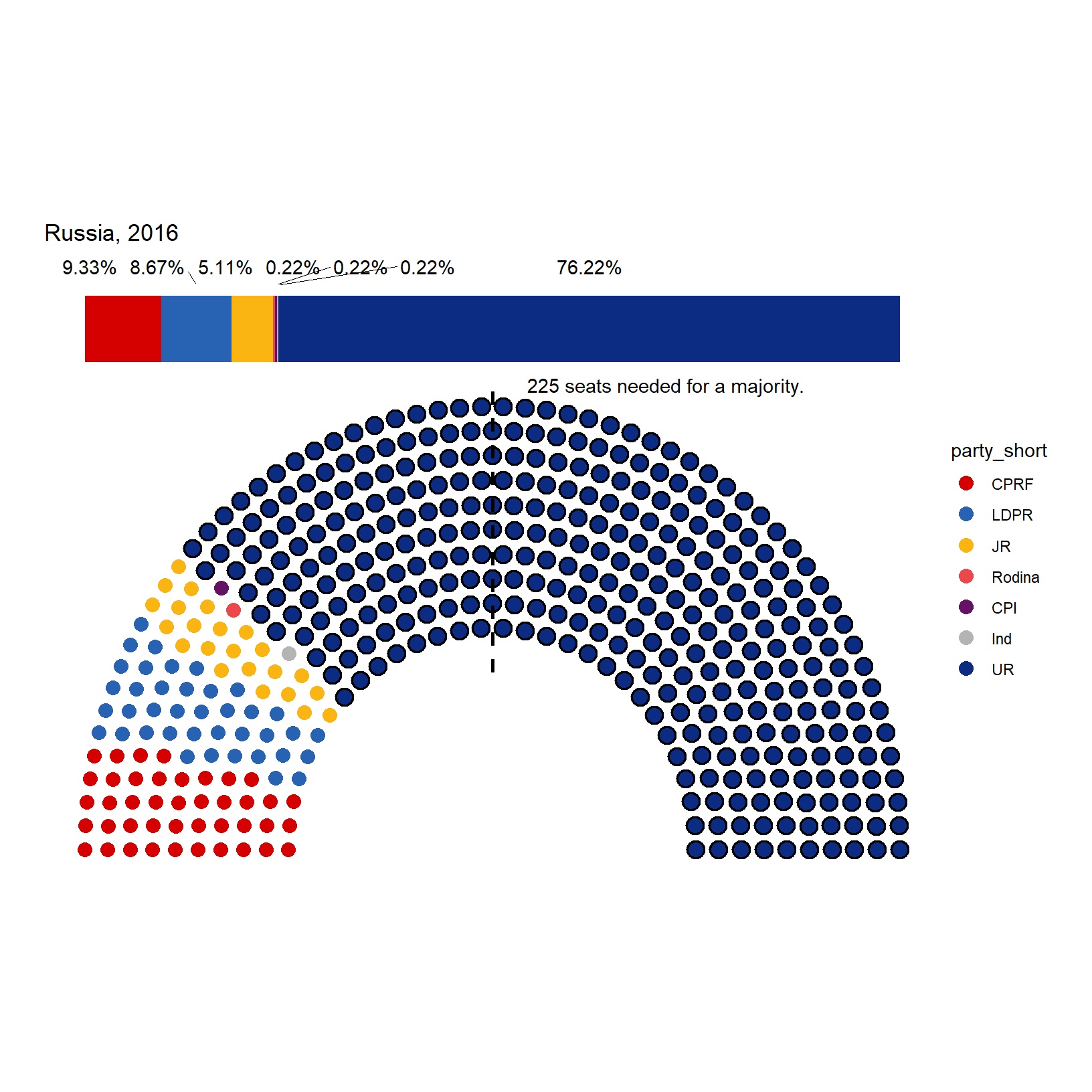
Parliament diagram with ggparliament
![Parliament diagram in ggplot2 with ggparliament]()
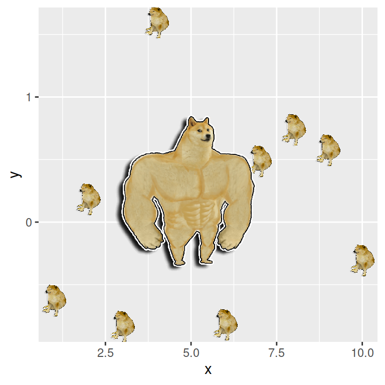
Adding dogs to ggplot2 with ggdogs
![Adding dogs to ggplot2 with ggdogs]()
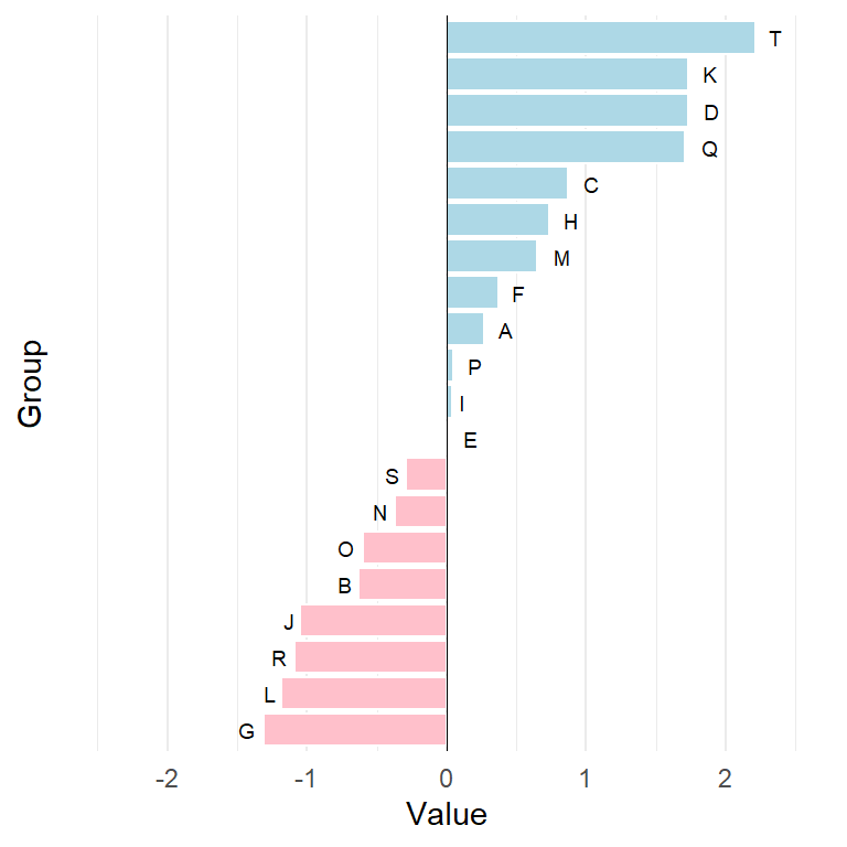
Diverging bar chart
![Diverging bar chart in ggplot2]()
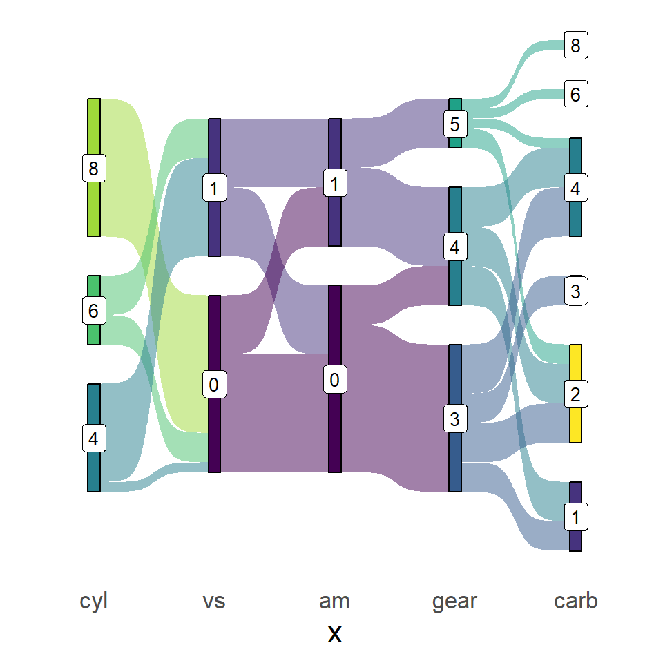
Sankey diagrams with ggsankey
![Sankey diagrams in ggplot2 with ggsankey]()
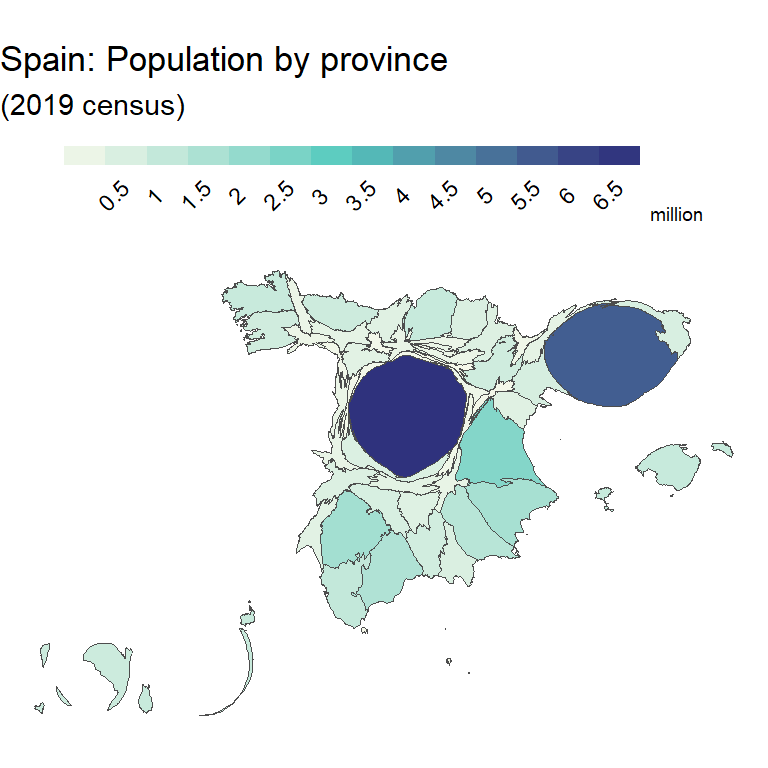
Cartograms
![Cartograms in ggplot2]()
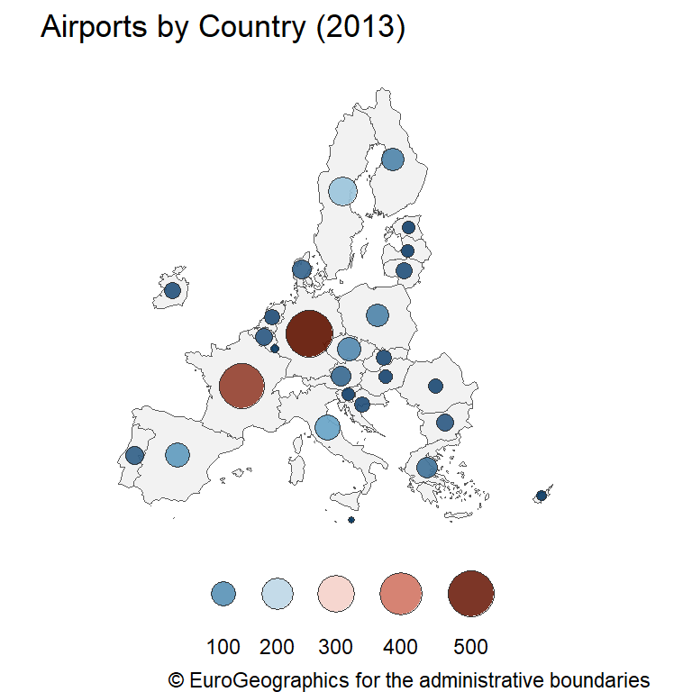
Proportional symbol maps
![Proportional symbol maps in ggplot2]()
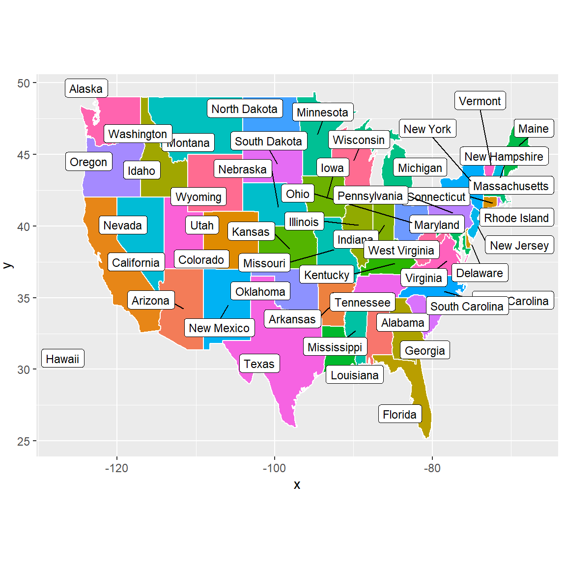
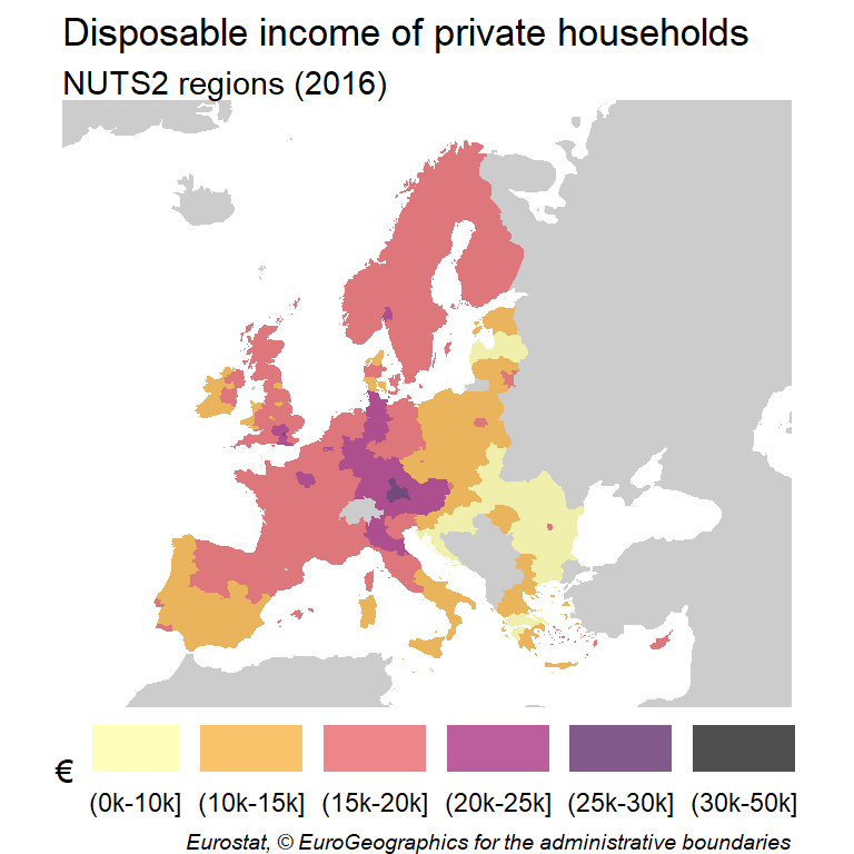
Choropleth maps
![Choropleth maps in ggplot2]()
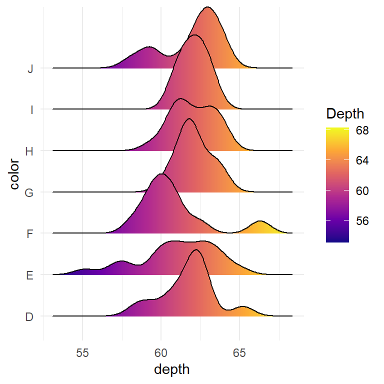
Ridgeline plot with ggridges
![Ridgeline plot in ggplot2 with ggridges]()
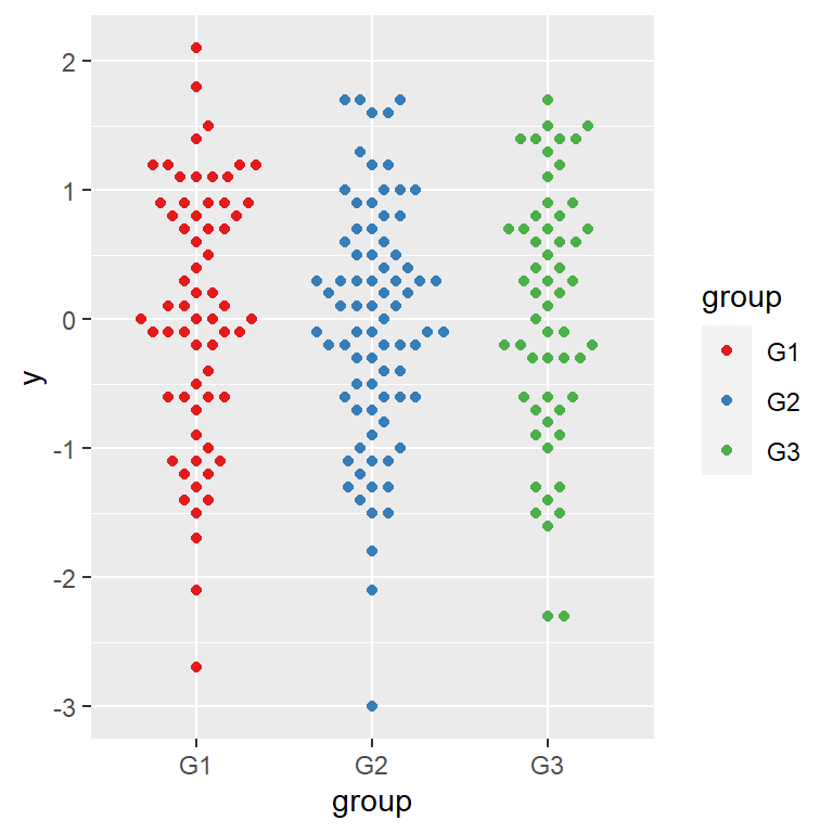
Beeswarm with ggbeeswarm
![Beeswarm in ggplot2 with ggbeeswarm]()
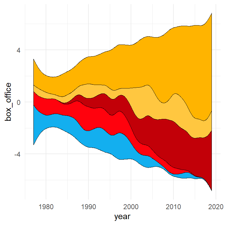
Streamgraph
![Streamgraph in ggplot2]()
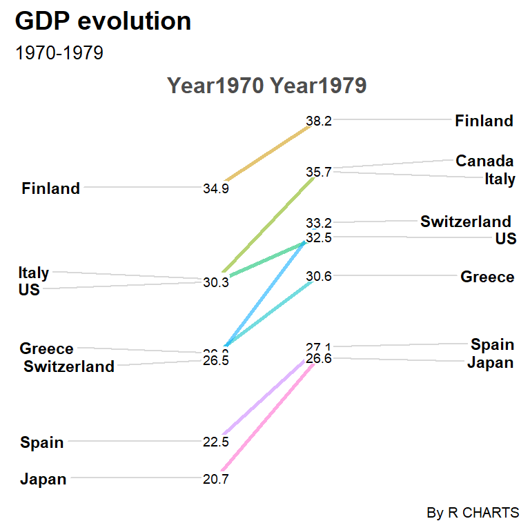
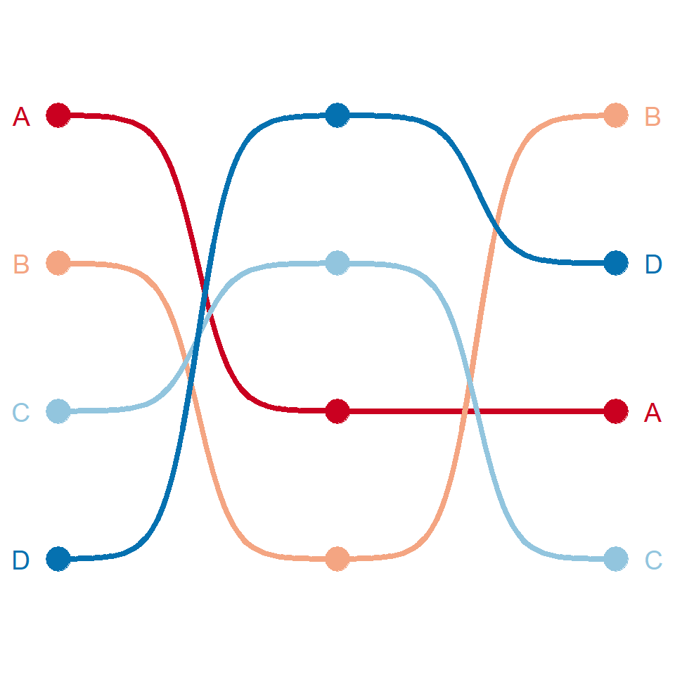
Slopegraph
![Slopegraph in ggplot2]()
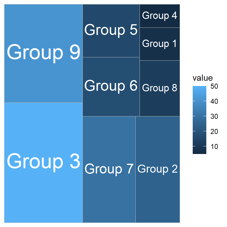
Treemaps with treemapify
![Treemaps in ggplot2 with treemapify]()
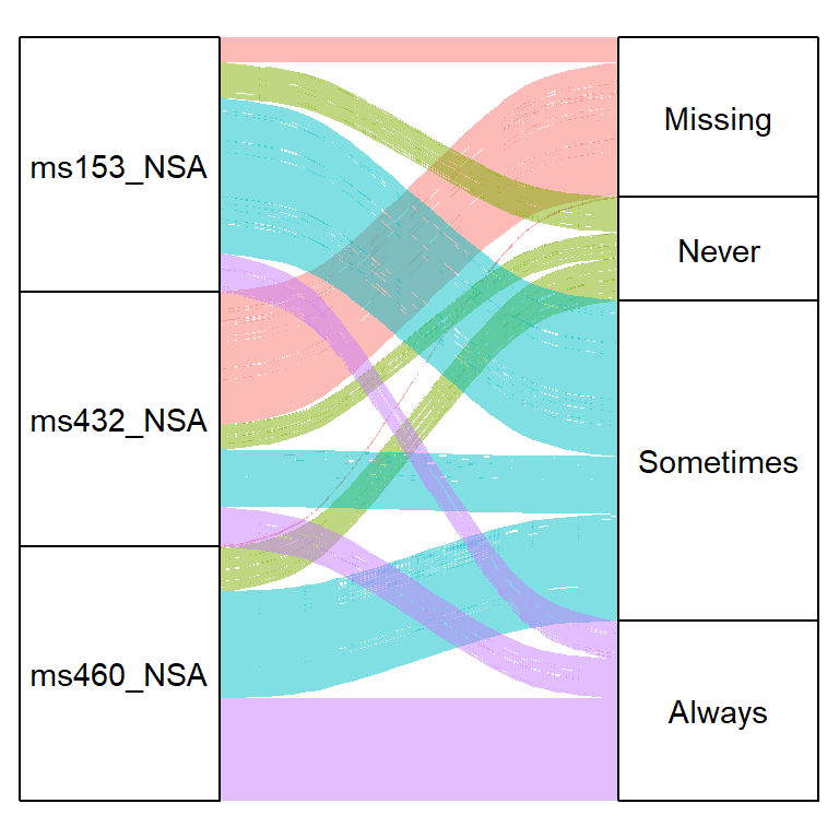
Alluvial plot with ggalluvial
![Alluvial plot in ggplot2 with ggalluvial]()
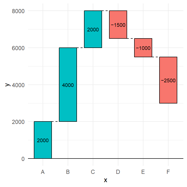
Waterfall charts with waterfalls package
![Waterfall charts in ggplot2 with waterfalls package]()
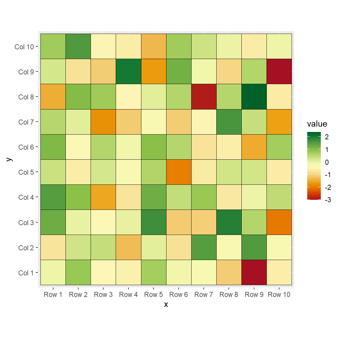
Heat map
![Heat map in ggplot2]()
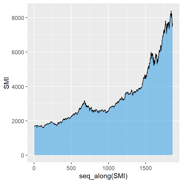
Area chart with geom_area
![Area chart in ggplot2 with geom_area]()
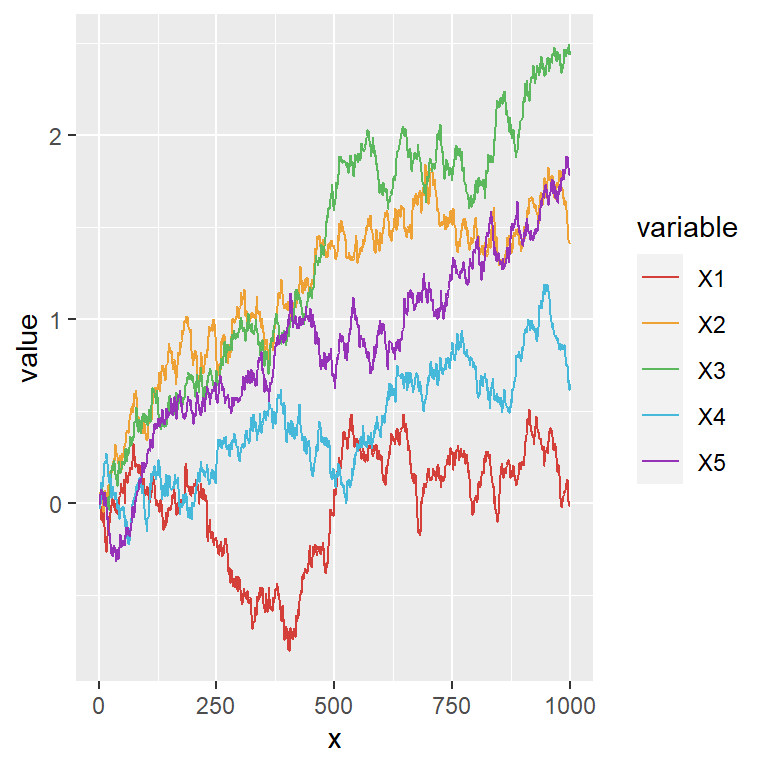
Line graph with multiple lines
![Line graph with multiple lines in ggplot2]()
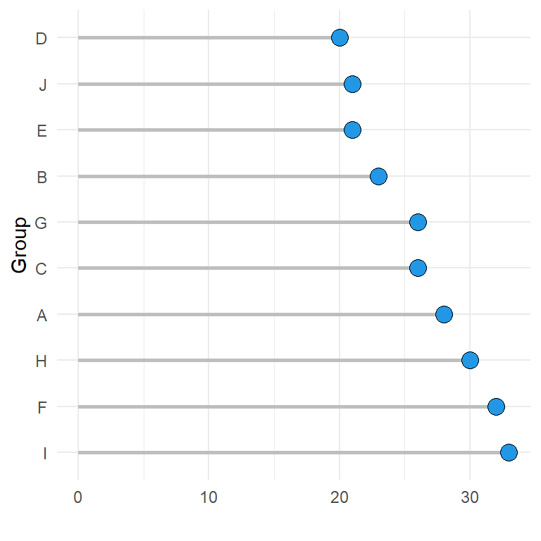
Lollipop chart
# Sample data set set.seed(1) df <- data.frame(x = LETTERS[1:10], y = sample(20:35, 10, replace = TRUE)) library(ggplot2) ggplot(df, aes(x = x, y = y)) + geom_segment(aes(x = x, xend = x, y = 0, yend = y)) + geom_point() ggplot(df, aes(x = x, y = y)) + geom_segment(aes(x = x, xend = x, y = 0, yend = y)) + geom_point() + coord_flip() ggplot(df, aes(x = x, y = y)) + geom_segment(aes(x = x, xend = x, y = 0, yend = y)) + geom_point(size = 4, pch = 21, bg = 4, col = 1) + coord_flip() ggplot(df, aes(x = x, y = y)) + geom_segment(aes(x = x, xend = x, y = 0, yend = y), color = "gray", lwd = 1.5) + geom_point(size = 4, pch = 21, bg = 4, col = 1) + coord_flip() ggplot(df, aes(x = x, y = y)) + geom_segment(aes(x = x, xend = x, y = 0, yend = y), color = "gray", lwd = 1) + geom_point(size = 4, pch = 21, bg = 4, col = 1) + scale_x_discrete(labels = paste0("G_", 1:10)) + coord_flip() ggplot(df, aes(x = x, y = y)) + geom_segment(aes(x = x, xend = x, y = 0, yend = y), color = "gray", lwd = 1) + geom_point(size = 4, pch = 21, bg = 4, col = 1) + scale_x_discrete(labels = paste("Group", 1:10)) + theme(axis.text.x = element_text(angle = 90, vjust = 0.5, hjust = 1)) ggplot(df, aes(x = x, y = y)) + geom_segment(aes(x = x, xend = x, y = 0, yend = y), color = "gray", lwd = 1) + geom_point(size = 4, pch = 21, bg = 4, col = 1) + scale_x_discrete(labels = paste0("G_", 1:10)) + coord_flip() + theme_minimal() ggplot(df, aes(x = x, y = y)) + geom_segment(aes(x = x, xend = x, y = 0, yend = y), color = "gray", lwd = 1) + geom_point(size = 7.5, pch = 21, bg = 4, col = 1) + geom_text(aes(label = y), color = "white", size = 3) + scale_x_discrete(labels = paste0("G_", 1:10)) + coord_flip() + theme_minimal() ggplot(df, aes(x = reorder(x, -y), y = y)) + geom_segment(aes(x = reorder(x, -y), xend = reorder(x, -y), y = 0, yend = y), color = "gray", lwd = 1) + geom_point(size = 4, pch = 21, bg = 4, col = 1) + xlab("Group") + ylab("") + coord_flip() + theme_minimal()
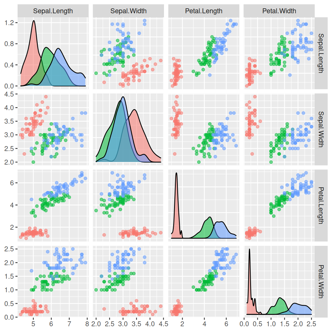
Pairs plot with ggpairs
![Pairs plot with ggpairs]()
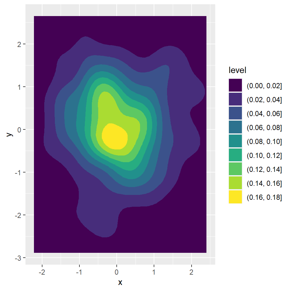
2D density contour plots
![2D density contour plots in ggplot2]()
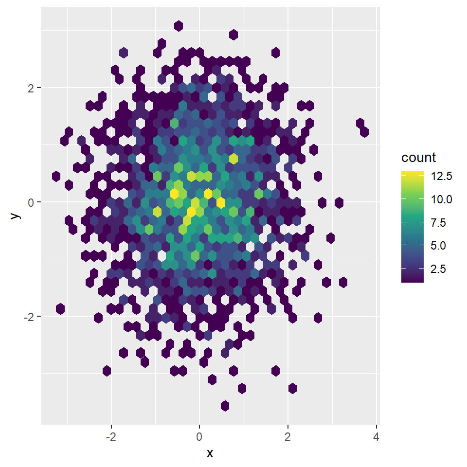
Hexbin chart
set.seed(1) df <- data.frame(x = rnorm(2000), y = rnorm(2000)) ggplot(df, aes(x = x, y = y)) + geom_hex() ggplot(df, aes(x = x, y = y)) + geom_hex(bins = 15) ggplot(df, aes(x = x, y = y)) + geom_hex(bins = 60) ggplot(df, aes(x = x, y = y)) + geom_hex(color = "white") ggplot(df, aes(x = x, y = y)) + geom_hex(color = 1, fill = 4, alpha = 0.4) ggplot(df, aes(x = x, y = y)) + geom_hex() + scale_fill_viridis_c() ggplot(df, aes(x = x, y = y)) + geom_hex() + guides(fill = guide_colourbar(barwidth = 0.7, barheight = 15)) ggplot(df, aes(x = x, y = y)) + geom_hex() + guides(fill = guide_colourbar(title = "Count")) ggplot(df, aes(x = x, y = y)) + geom_hex() + guides(fill = guide_colourbar(label = FALSE, ticks = FALSE)) ggplot(df, aes(x = x, y = y)) + geom_hex() + theme(legend.position = "none")
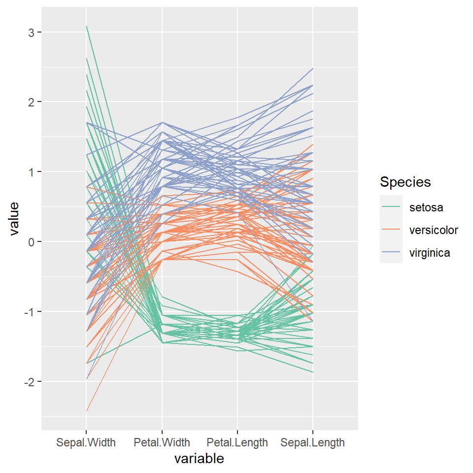
Parallel coordinates with ggparcoord
![Parallel coordinates in ggplot2 with ggparcoord]()
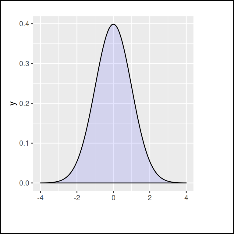
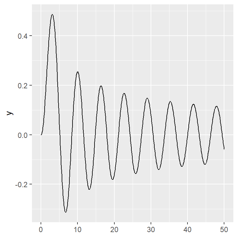
Drawing functions with geom_function
![Drawing functions in ggplot2 with geom_function]()
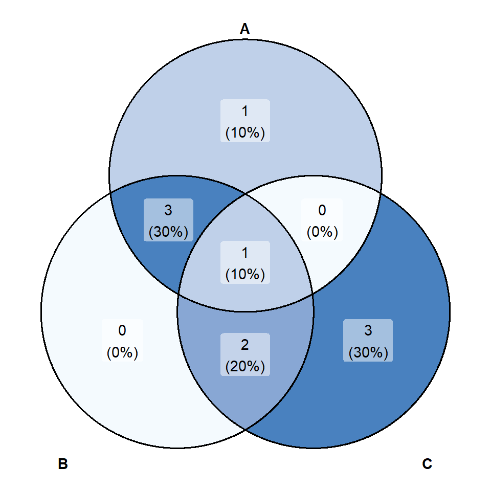
Venn diagram
![Venn diagram in ggplot2]()
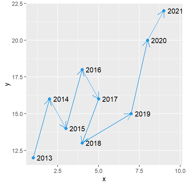
Connected scatter plot
![Connected scatter plot in ggplot2]()
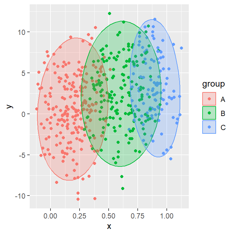
Scatter plot with ellipses
![Scatter plot with ellipses in ggplot2]()
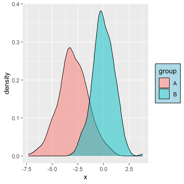
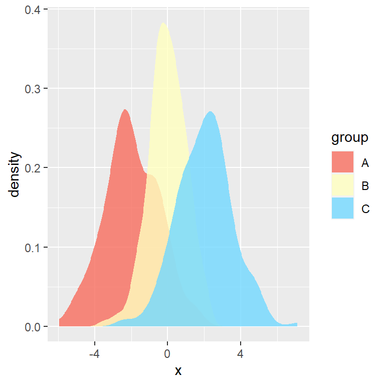
Density plot by group
![Density plot by group in ggplot2]()
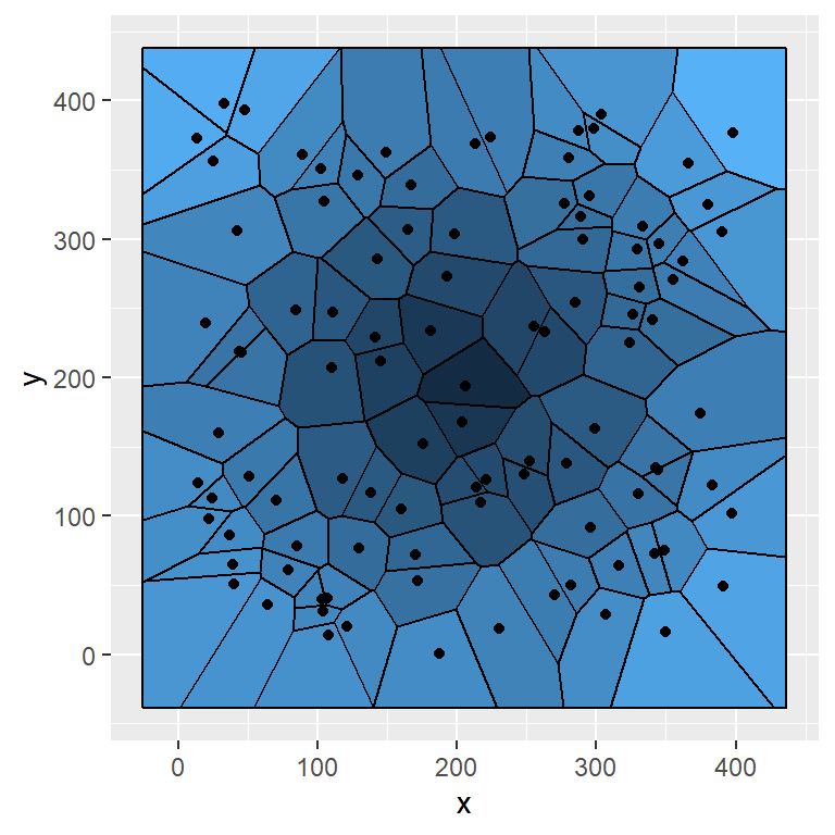
Voronoi diagram with ggvoronoi
![Voronoi diagram in ggplot2 with ggvoronoi]()
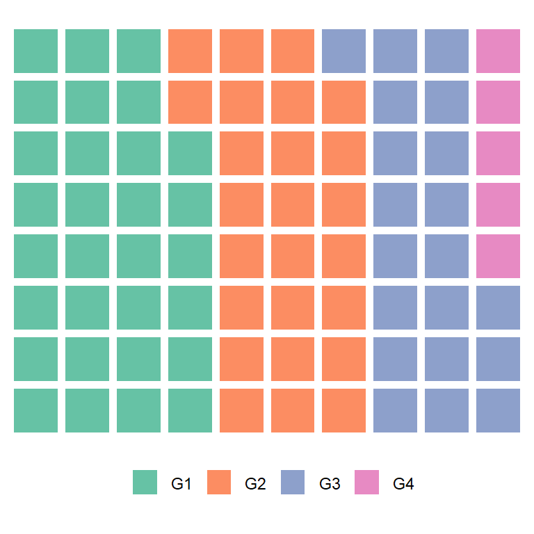
Waffle chart (square pie)
![Waffle chart (square pie) in ggplot2]()
Bump chart with ggbump
install.packages("tidyverse") install.packages("ggbump") library(tidyverse) library(ggbump) year <- rep(2019:2021, 4) position <- c(4, 2, 2, 3, 1, 4, 2, 3, 1, 1, 4, 3) player <- c("A", "A", "A","B", "B", "B", "C", "C", "C","D", "D", "D") df <- data.frame(x = year, y = position, group = player) ggplot(df, aes(x = x, y = y, color = group)) + geom_bump() ggplot(df, aes(x = x, y = y, color = group)) + geom_bump(size = 1.5) + geom_point(size = 6) ggplot(df, aes(x = x, y = y, color = group)) + geom_bump(size = 1.5) + geom_point(size = 6) + scale_color_brewer(palette = "RdBu") ggplot(df, aes(x = x, y = y, color = group)) + geom_bump(size = 1.5) + geom_point(size = 6) + geom_text(data = df %>% filter(x == min(x)), aes(x = x - 0.1, label = group), size = 5, hjust = 1) + geom_text(data = df %>% filter(x == max(x)), aes(x = x + 0.1, label = group), size = 5, hjust = 0) + scale_color_brewer(palette = "RdBu") + theme_void() + theme(legend.position = "none")
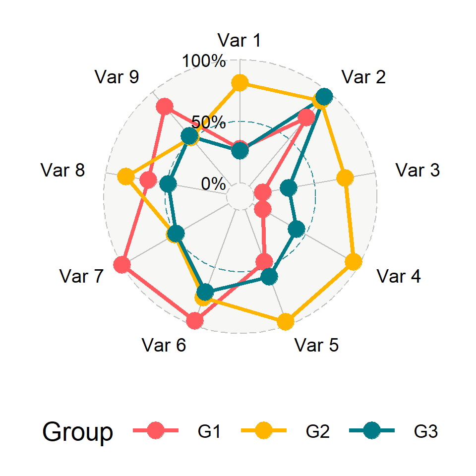
Radar chart with ggradar
![Radar chart in ggplot2 with ggradar]()
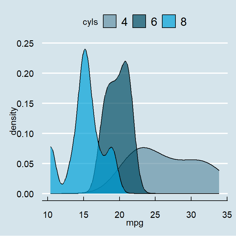
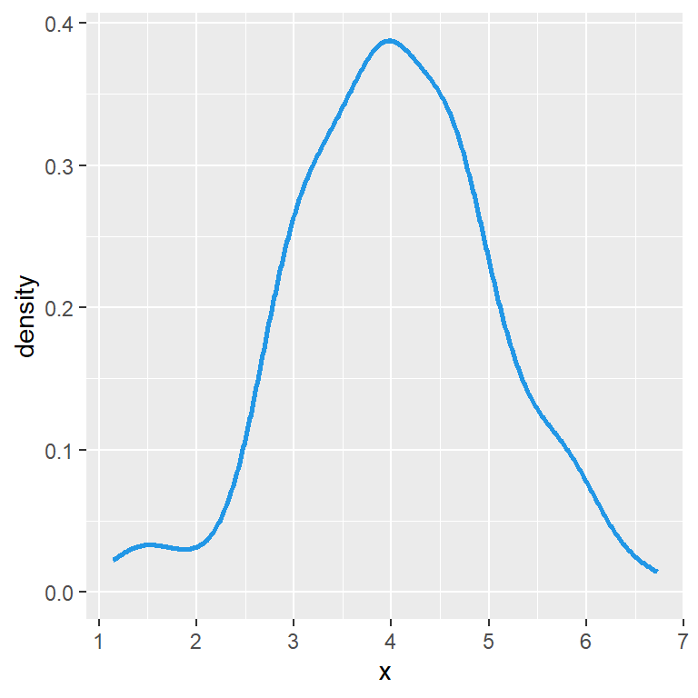
Density plot with geom_density
![Density plot in ggplot2 with geom_density]()
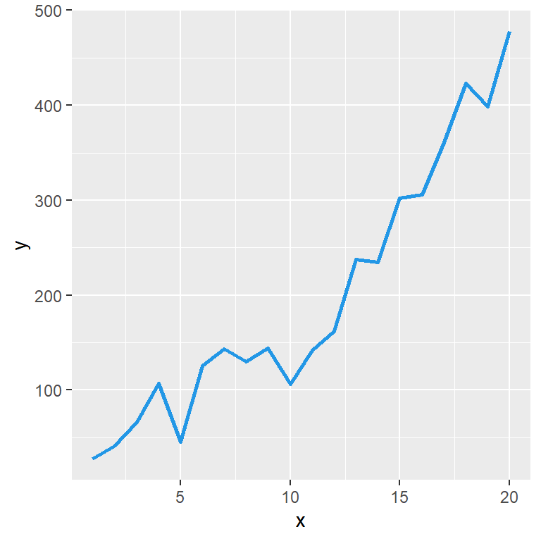
Line graph
![Line graph in ggplot2]()
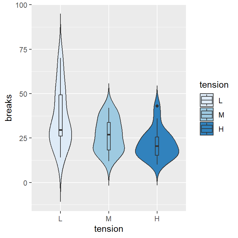
Violin plot by group
![Violin plot by group in ggplot2]()
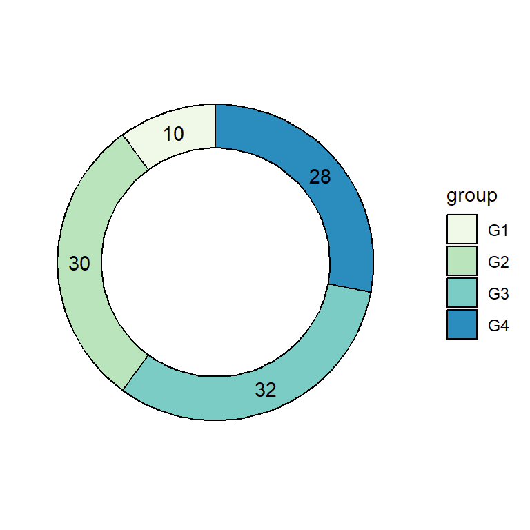
Donut chart
![Donut chart in ggplot2]()
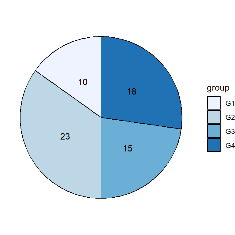
Pie chart
![Pie chart in ggplot2]()
Pie chart with labels outside
![Pie chart with labels outside in ggplot2]()
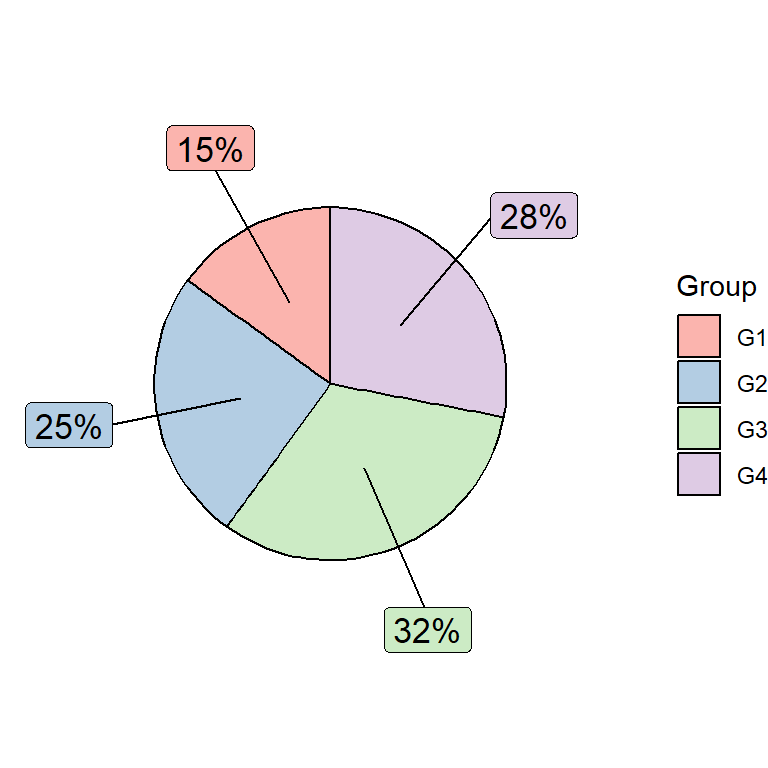
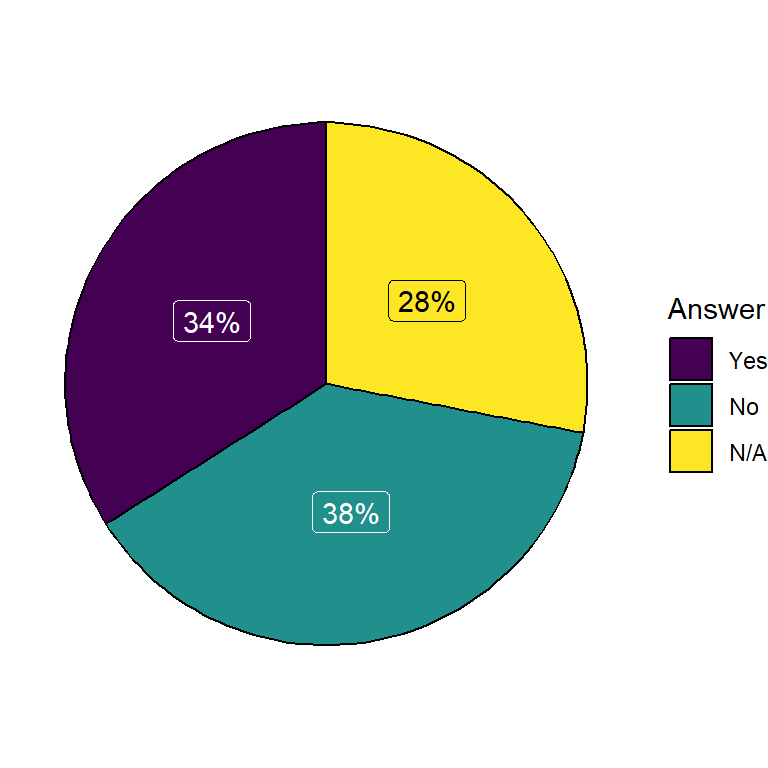
Pie chart with percentages
![Pie chart with percentages in ggplot2]()
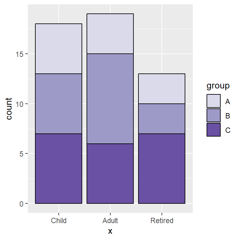
Stacked bar chart
![Stacked bar chart in ggplot2]()
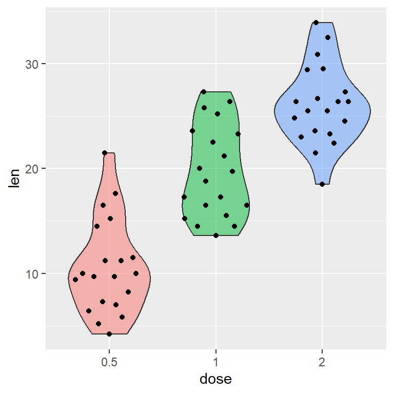
Violin plot with data points
![Violin plot with data points in ggplot2]()
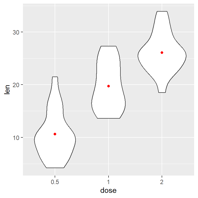
Violin plot with mean
![Violin plot with mean in ggplot2]()
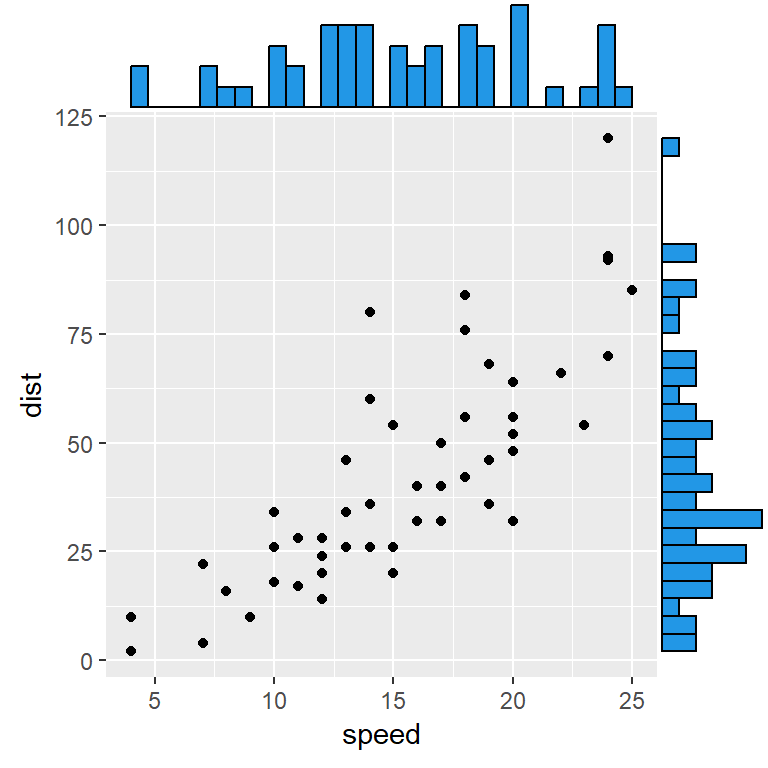
Scatter plot with marginal histograms
![Scatter plot with marginal histograms in ggplot2]()
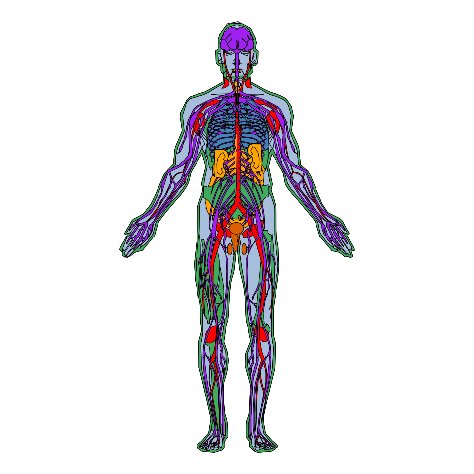
Anatogram images with gganatogram
![Anatogram images in ggplot2 with gganatogram]()
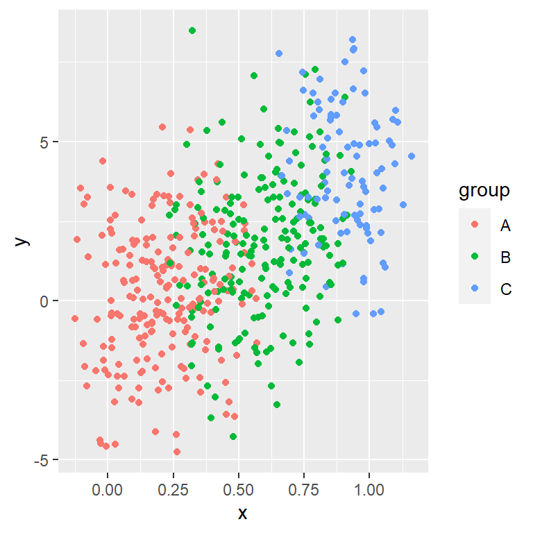
Scatter plot by group
![Scatter plot by group in ggplot2]()
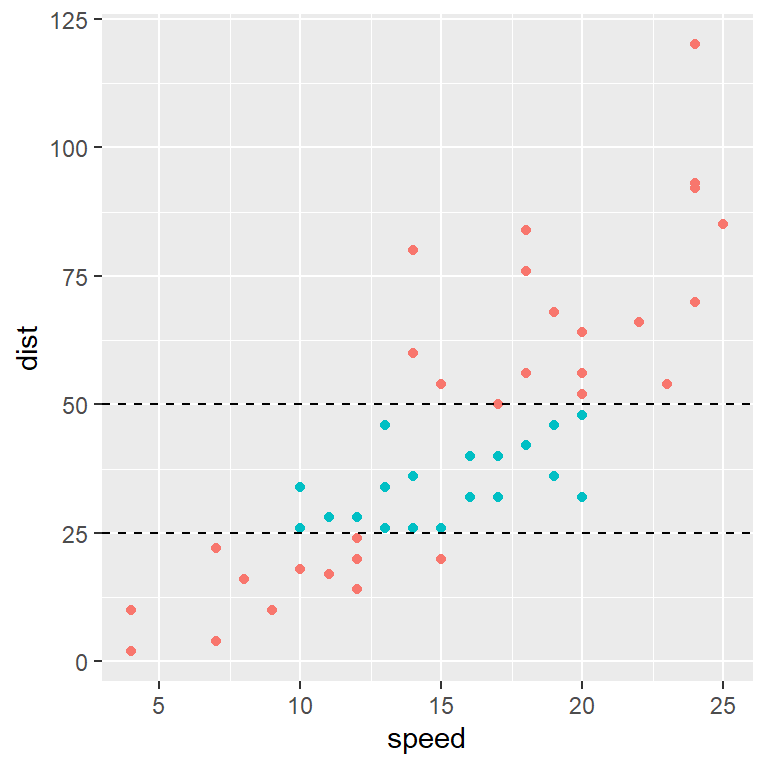
Scatter plot
![Scatter plot in ggplot2]()
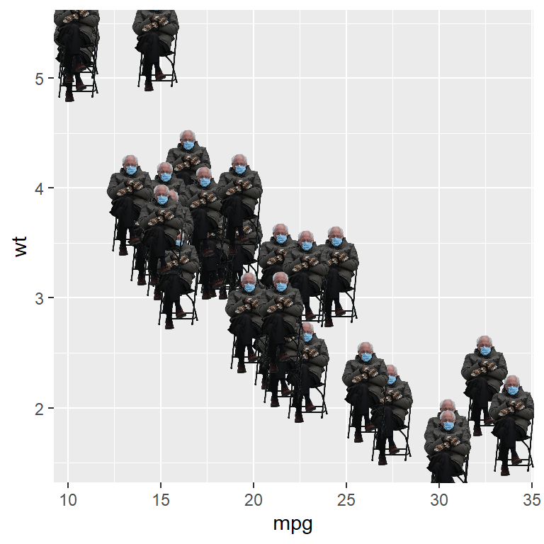
Adding Bernie Sanders to ggplot2
![Adding Bernie Sanders to ggplot2]()
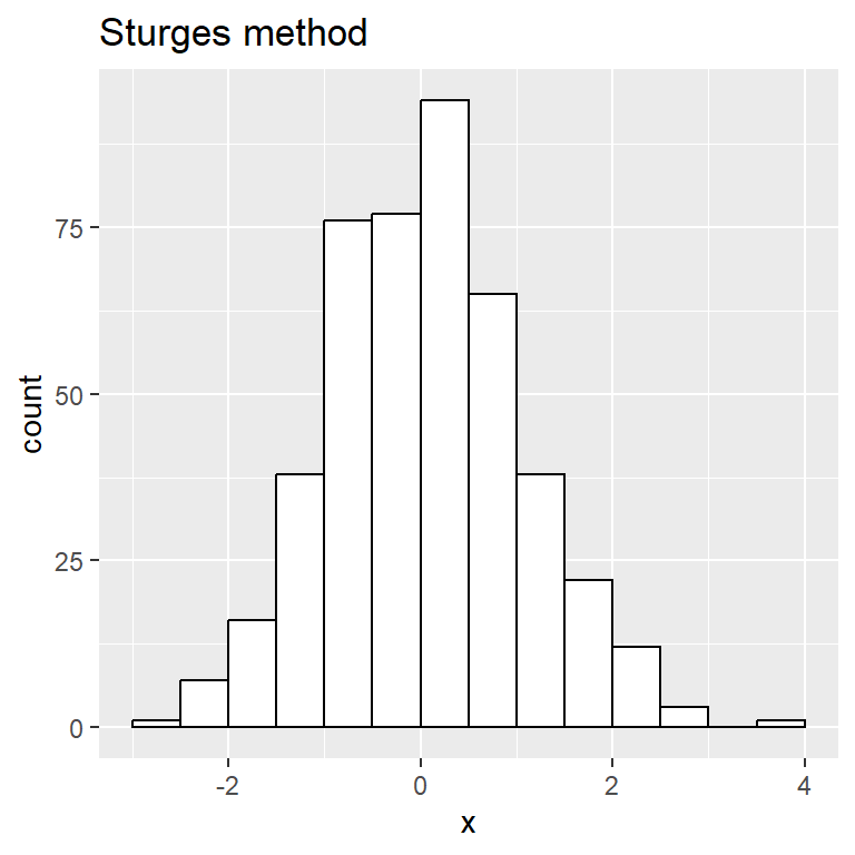
Histogram with Sturges method
![Histogram in ggplot2 with Sturges method]()
LEGO mosaics in R with brickr
![LEGO mosaics in R with brickr]()
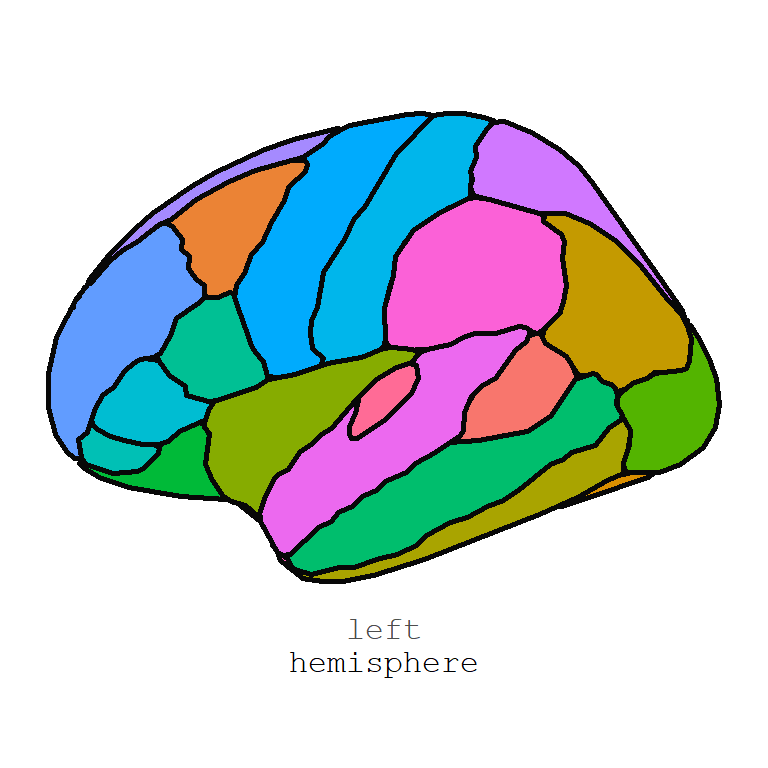
Plotting brain atlases with ggseg
![Plotting brain atlases in ggplot2 with ggseg]()
Adding cats to ggplot2 with ggcats
![Adding cats to ggplot2 with ggcats]()
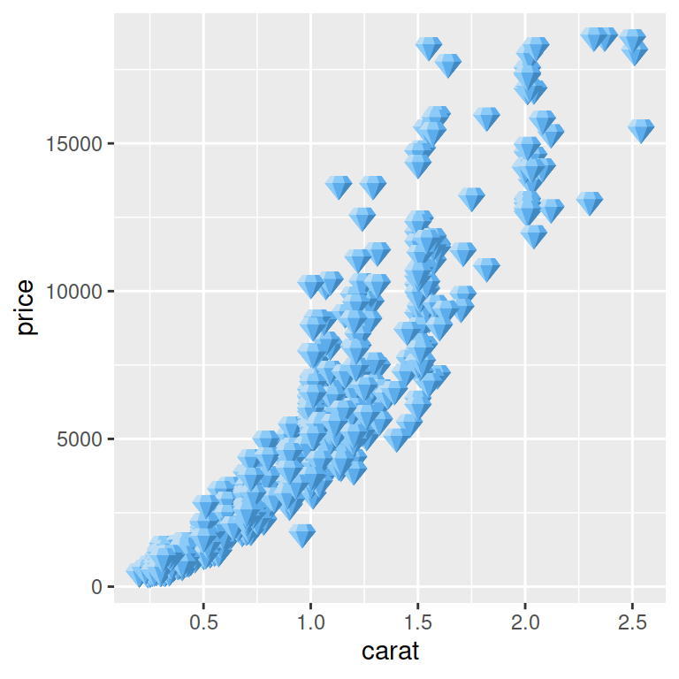
Adding emojis to ggplot2 with emoGG
![Adding emojis to ggplot2 with emoGG]()
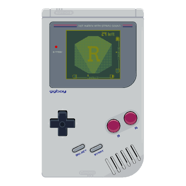
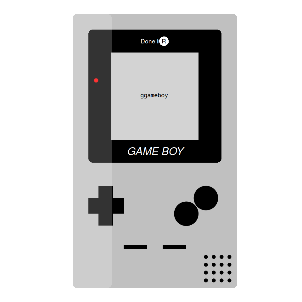
Game Boy screen simulator with ggboy
![Game Boy screen simulator in ggplot2 with ggboy]()
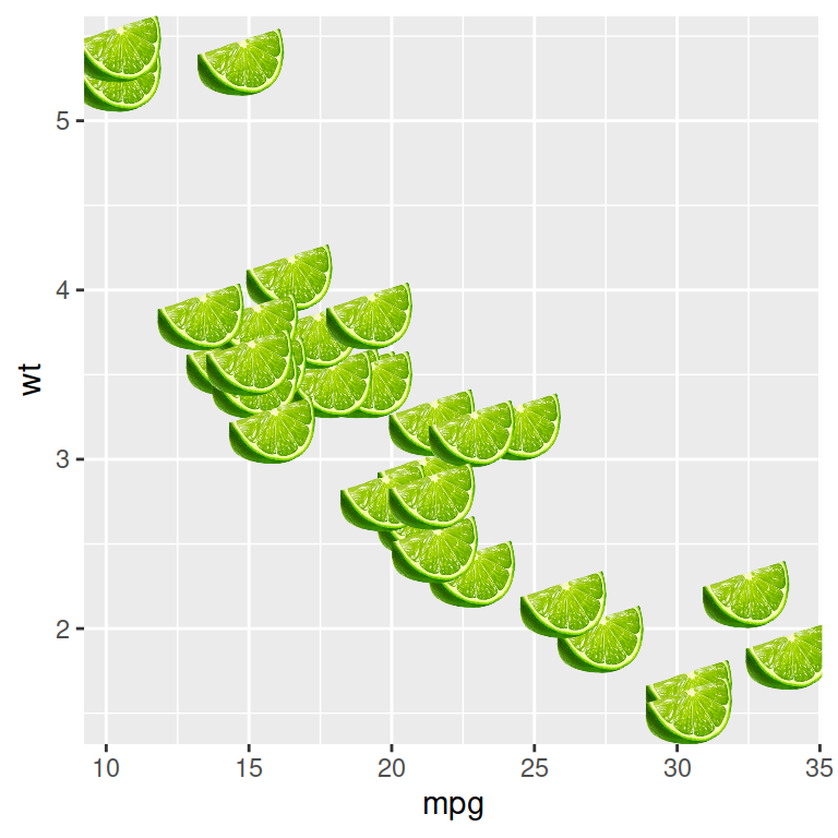
geom_lime and geom_pint
![geom_lime and geom_pint]()
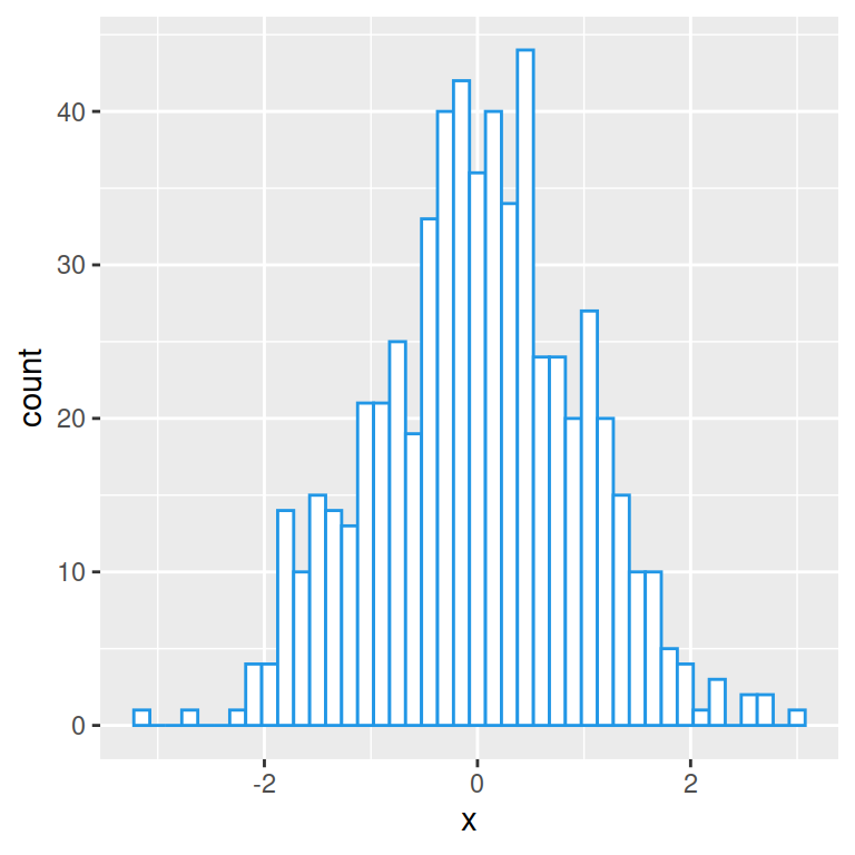
Histogram bins and binwidth
![Histogram bins and binwidth in ggplot2]()
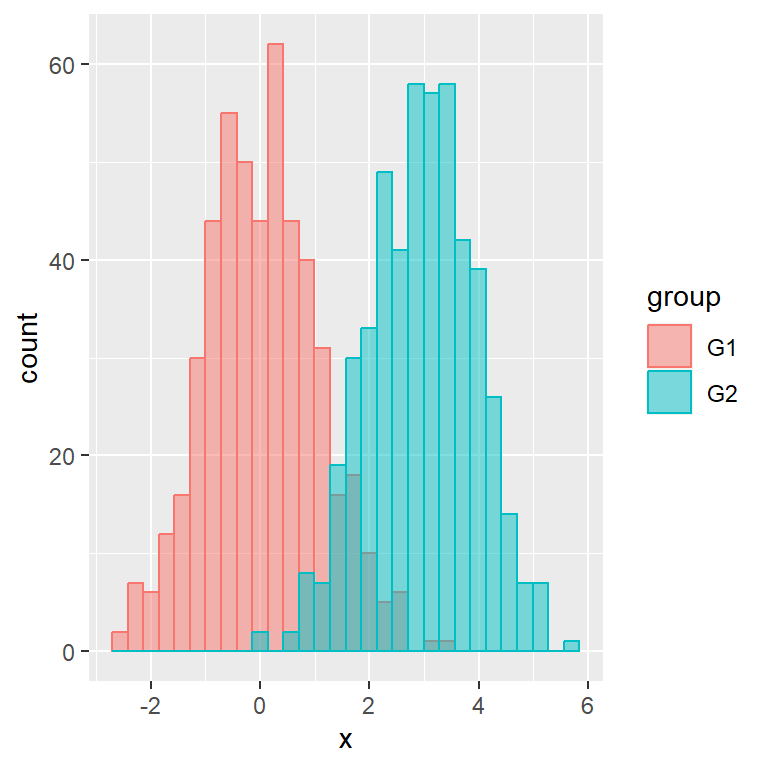
Histogram by group
![Histogram by group in ggplot2]()
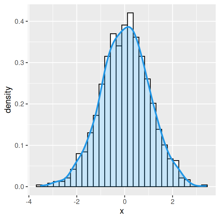
Histogram with density
![Histogram with density in ggplot2]()
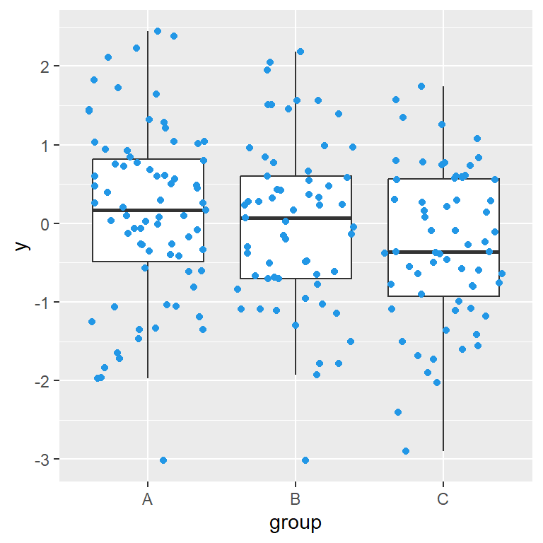
Box plot with jittered data points
![Box plot with jittered data points in ggplot2]()
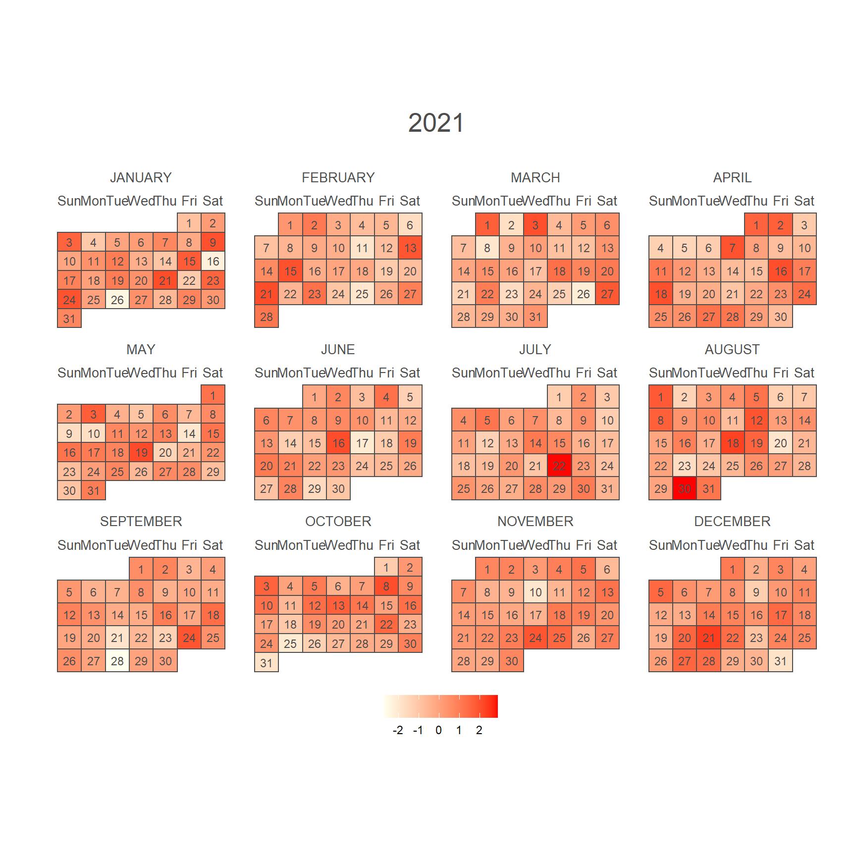
Yearly calendar heat map in R
![Yearly calendar heat map in R]()
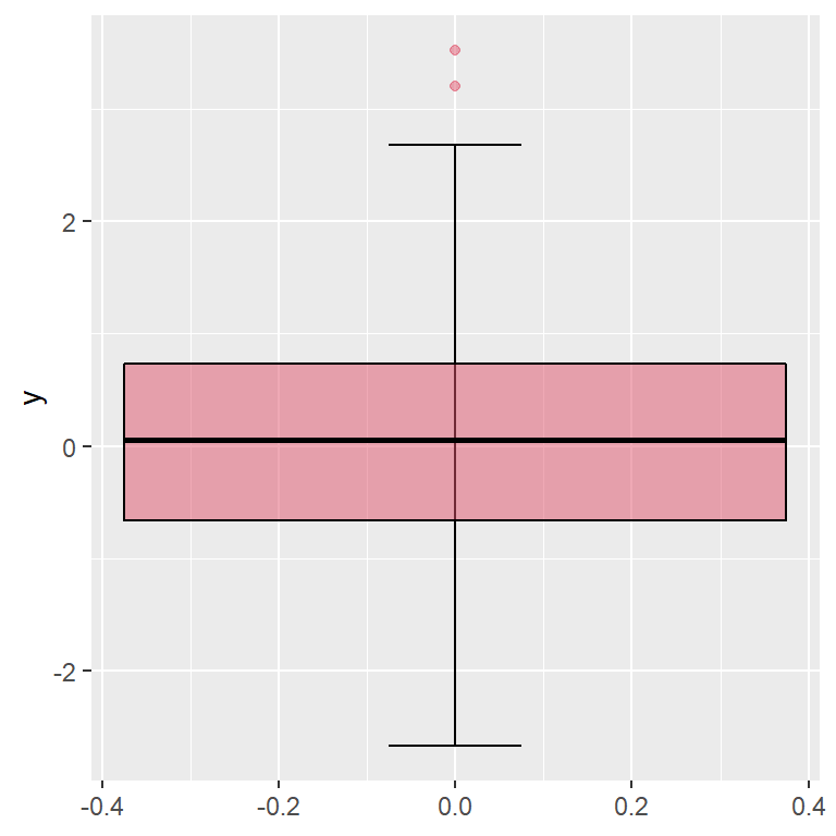
Box plot
![Box plot in ggplot2]()
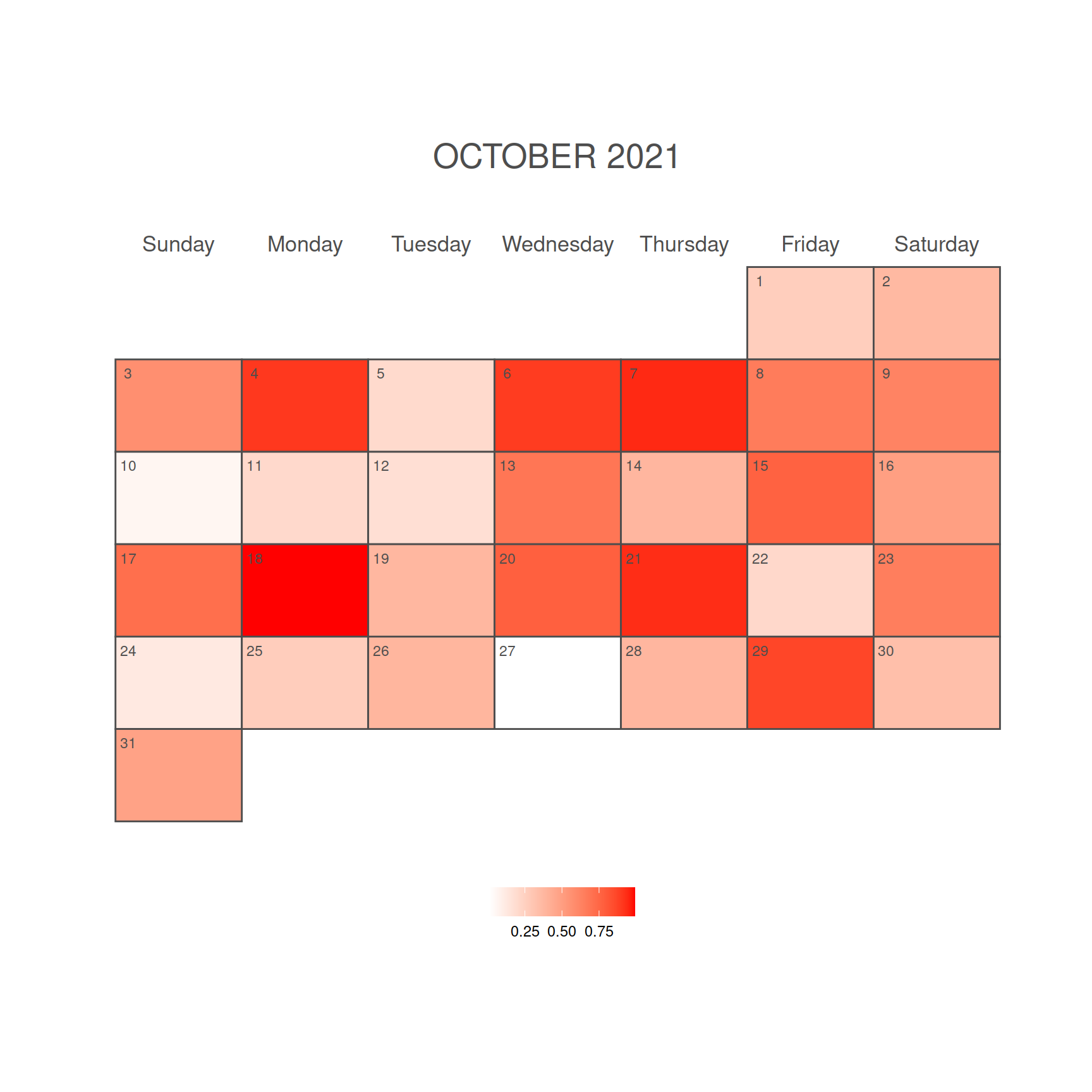
Monthly calendar heat map in R
![Monthly calendar heat map in R]()
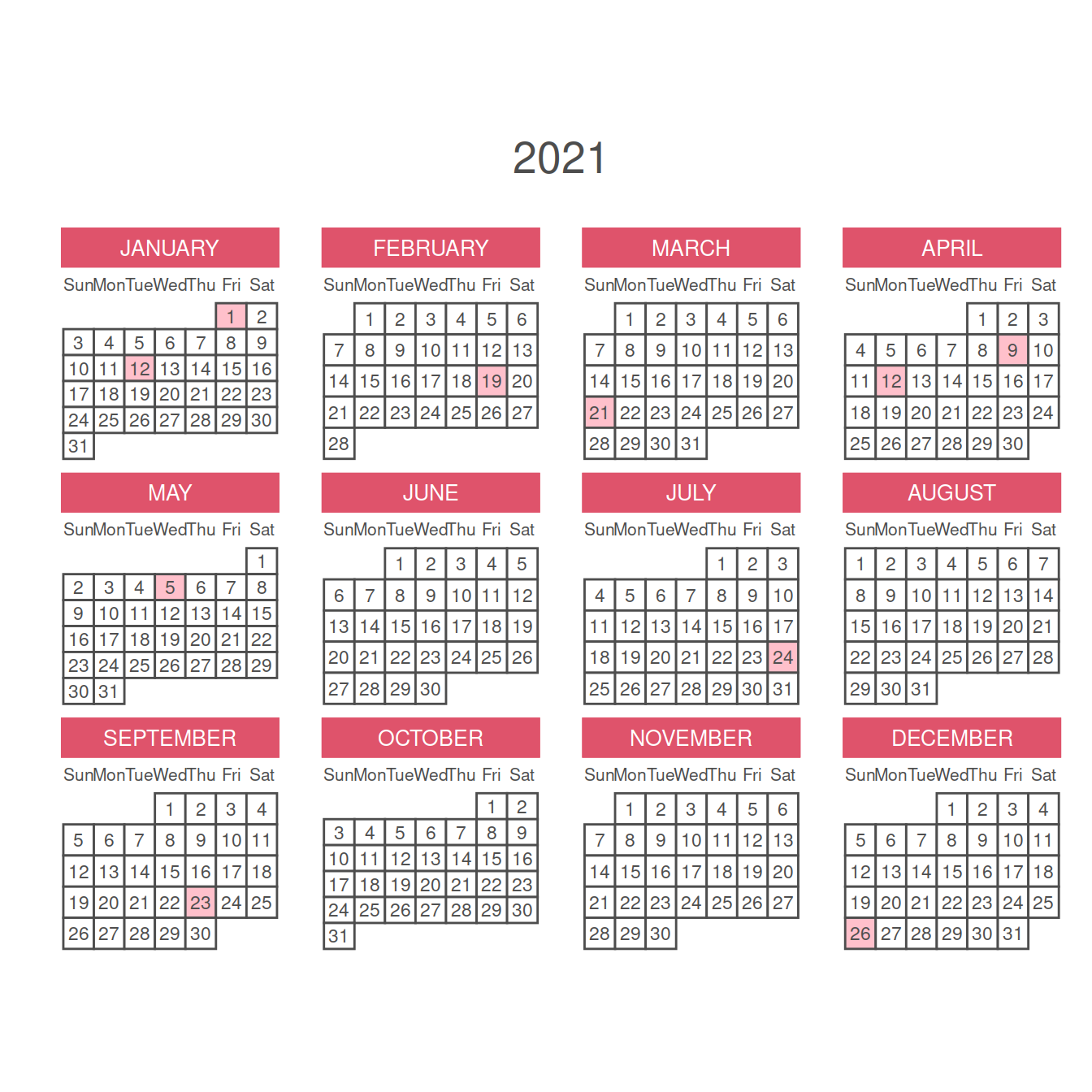
Yearly calendar
![Yearly calendar in ggplot2]()
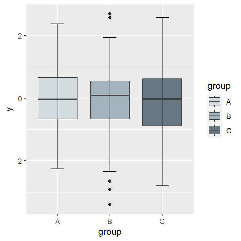
Box plot by group
![Box plot by group in ggplot2]()
Game boy
![Game boy in ggplot2]()
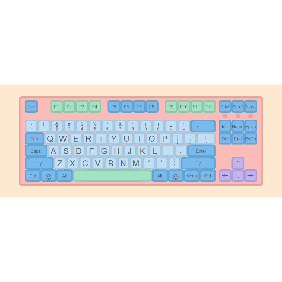
Keyboards with ggkeyboard
![Keyboards in ggplot2 with ggkeyboard]()
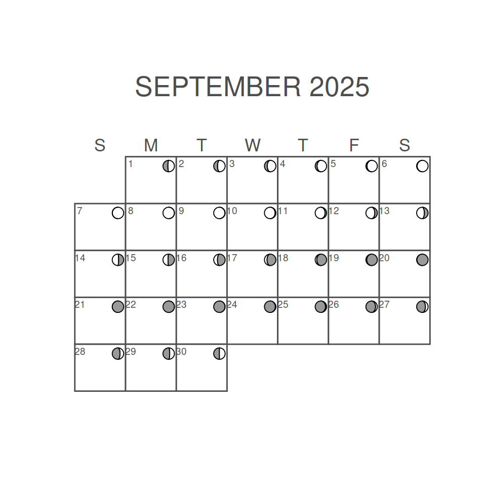
Lunar calendar with ggplot2
![Lunar calendar with ggplot2]()
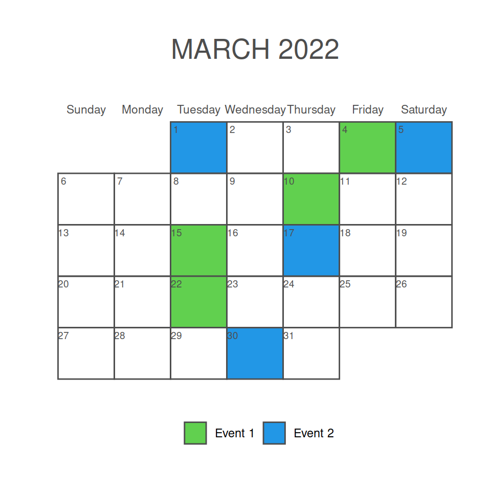
Monthly calendar
![Monthly calendar in ggplot2]()
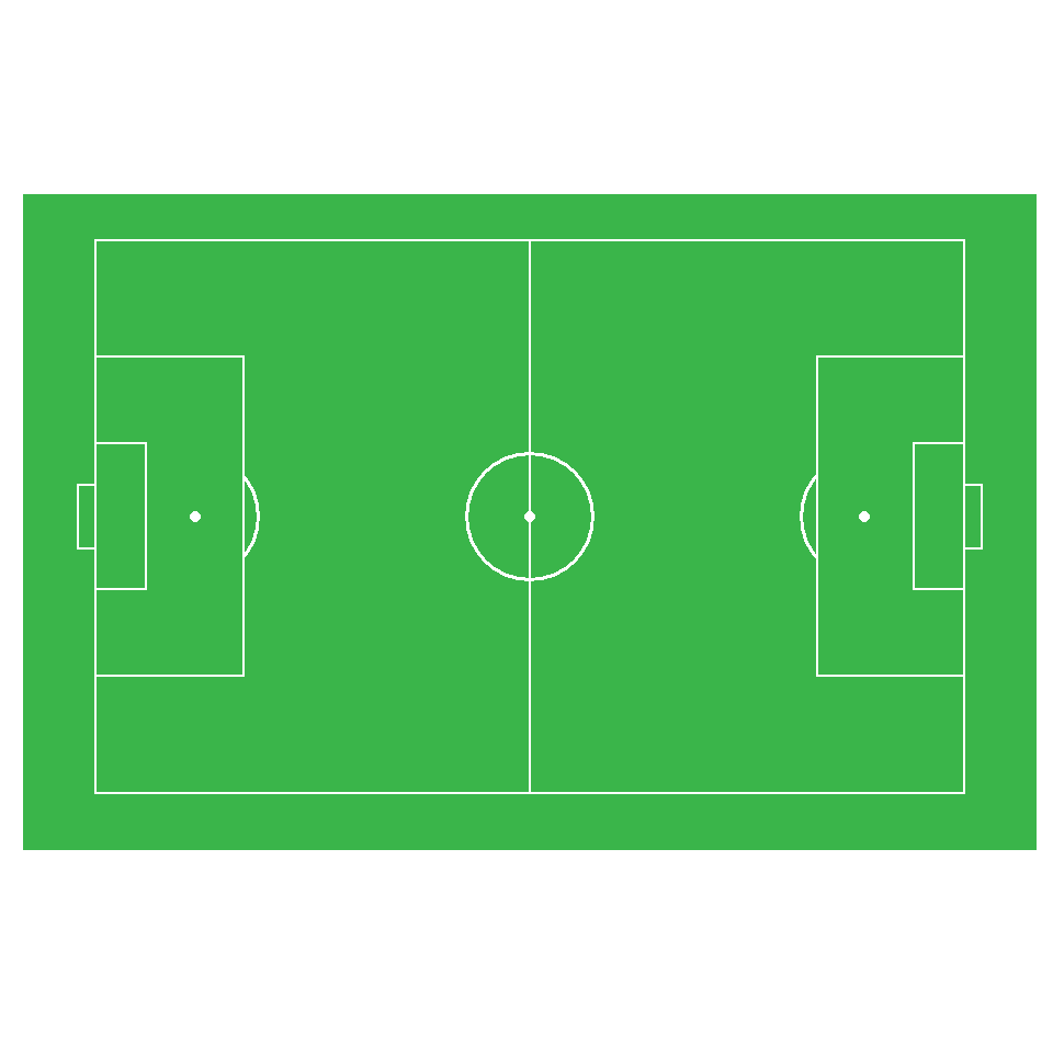
Soccer event data with ggsoccer
![Soccer event data in ggplot2 with ggsoccer]()